2.6 — Long Run Industry Equilibrium — Class Content
Contents
- Section 1: Monday, March 22, 2021
- Section 2: Tuesday, March 30, 2021Section 2, because of no class on Thursday Feb 18 and Tuesday Mar 9, is 2 classes behind Section 1.
Overview
We wrap up Unit 2 on Producers today (or finally finish it Wednesday), by bringing our optimization model of how firms maximize profits into the long run, when firms can enter or exit depending on profitability. We also now need to talk about the fact that our firm is not the only profit-maximizing firm in the market, so we derive an equilibrium model of the industry in the long run.
Famously, we see that in competitive industries, economic profits get driven to zero in the long run, as firms enter or exit any time there are profits or losses.
We also talk about the hard to understand, but extremely important, idea of economic rents.
Next class (Wednesday October 7) we will have a review session for Exam 2, which will be next week. We will not have class on Monday October 12) to give you a chance to work on the exam, and not be distracted by new material. We will begin Unit 3 on Wednesday October 14.
I have your Exam 1 graded and will discuss them at the end of class today. See assignments below for more information.
Readings
- Ch. 8.4-8.5, 2.5 in Goolsbee, Levitt, and Syverson, 2019
Slides
Assignments
Problem Set 4 Due Sun Mar 28/April 4
Problem set 4 (on 2.4-2.6) is due by 11:59 PM Sunday March 28 (Section 1 M/W) and Sunday April 4 (Section 2 Tu/Th) by PDF upload to Blackboard Assignments.
Exam 2
This is the final topic for Unit 2, which means we are ready for Exam 2. However, this semester has an awkward schedule, for two reasons: first is Section 2 is a full week behind Section 1 due to Spring Break days, and second is that next week is “Wellness week” and I cannot give an exam during that week. Thus:
- For Section 1 (M/W)
We will proceed with 3.1 and 3.2 for the next two classes (Wed Mar 24 and Mon Mar 29) and have a review session on Wed Mar 31 for Exam 2. Topics 3.1 and 3.2 will not be on Exam 2, but will be on the Final Exam.
- For Section 2 (Tu/Th)
We will catch up and finish 2.6 on Tues Mar 30, and have a review session on Thur April 1.
Both sections will have Exam 2 the week of April 5.
Appendix
Producer Surplus
You may recall from principles of microeconomics the concepts of consumer surplus and producer surplus in markets. While we will study them in our next unit with Supply & Demand, we can talk about the producer surplus to each firm here.
Producer surplus essentially measures the “gains from exchange” to each party — for a producer, it is how much they benefit (on net) from selling their output.
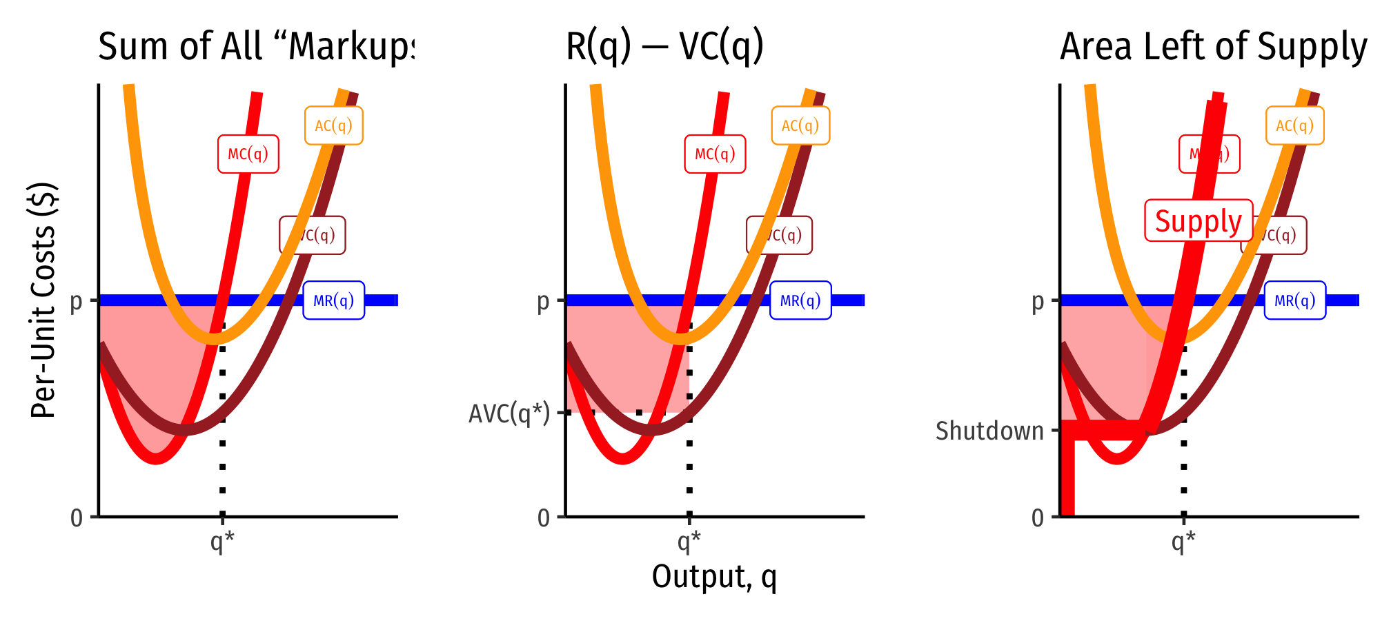
There are three equivalent ways of visualizing and measuring producer surplus for a firm. I will begin with a generalized series of cost curves:

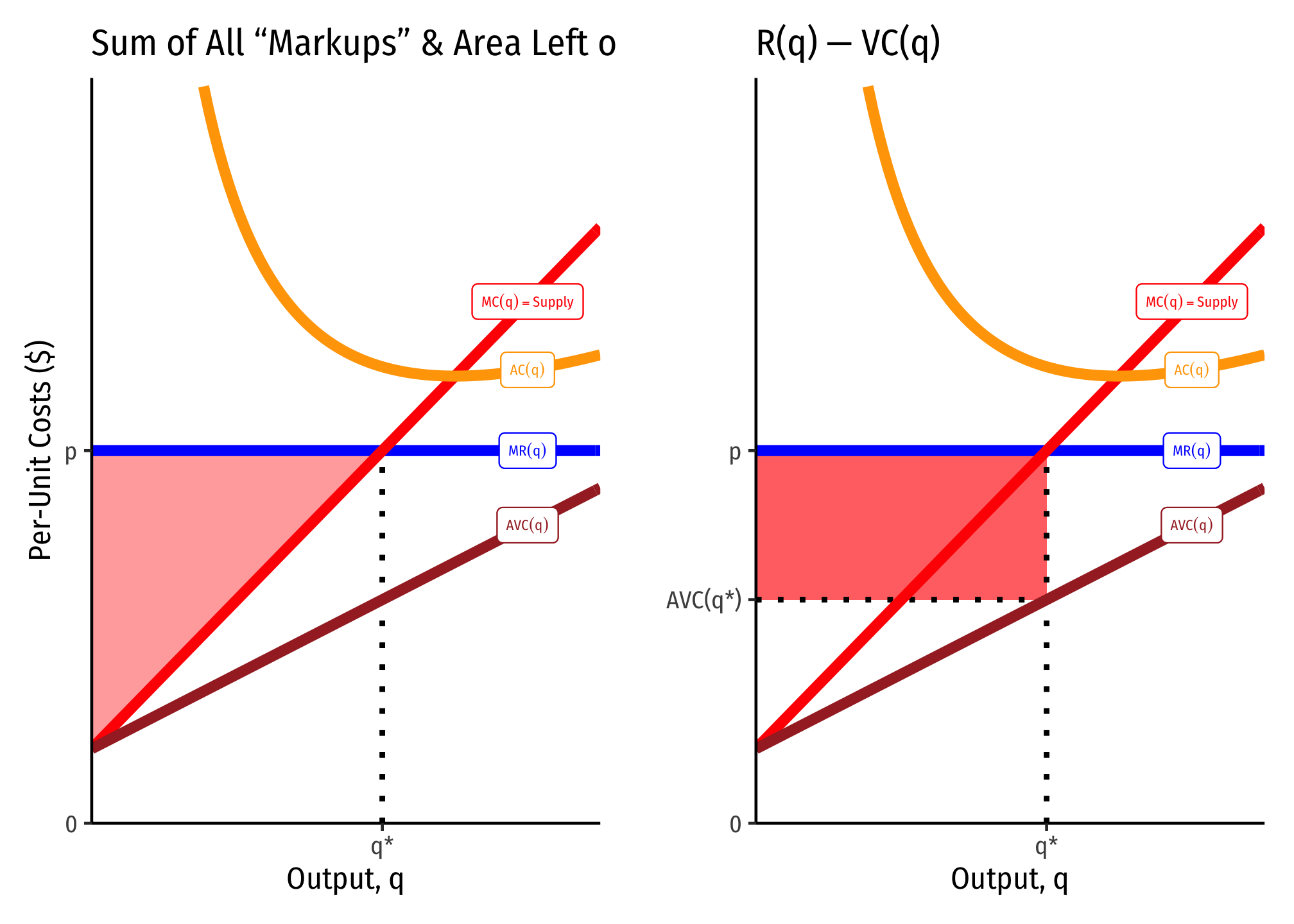
These often converge, and are also easier to identify when marginal cost is linear (and thus, average variable cost is also linear, and starts at the same point as marginal cost, the shutdown price). Here it producer surplus becomes the familiar “triangle” between the market price and the supply curve. Note we can also calculate it as the rectangle of revenues minus variable costs (right).

What’s the Difference Between Producer Surplus and Profit?
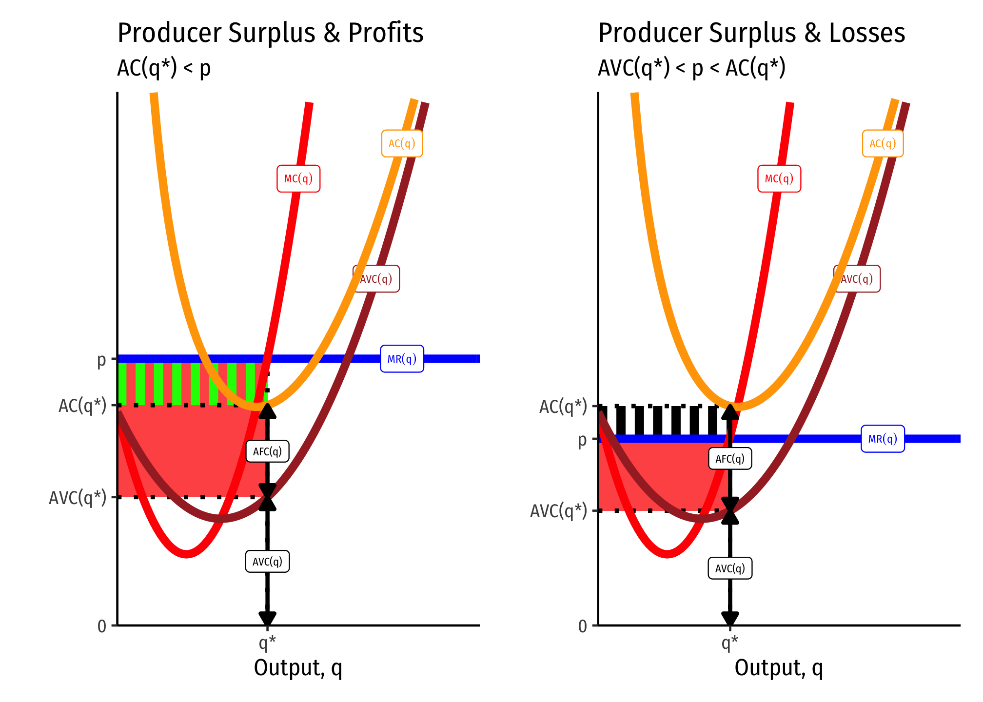
Producer surplus (PS) looks a lot like profits \((\pi)\), but they are in fact different:
\[\begin{align*} \color{red}{PS} &= R(q) - VC\\ & \\ \color{green}{\pi} & = R(q) - C(q) \\ \color{green}{\pi} &= R(q) - VC(q)-f\\ & \\ \color{green}{\pi}-\color{red}{PS}&=-f\\ \color{green}{\pi}&=\color{red}{PS}-f\\ \end{align*}\]
Producer surplus does not include fixed costs \((f)\), but profit \((\pi)\) does.
If there are no fixed costs, then producer surplus and profits are the same thing.
This leads to some other implications connected with the shutdown condition \(p<AVC(q)\). A firm will always earn producer surplus, but may earn losses (negative profit) so long as the price is above the shutdown price. This is because each unit of output sold generates at least enough revenues as (non-fixed) variable costs, \(pq \geq VC(q)\) or (dividing by \(q)\) \(p \geq AVC(q)\).
A firm will shut down production in the short run if it earning no producer surplus. This would happen if it earns fewer revenues than (non-fixed) variable costs: \(pq < VC(q)\) or (dividing by \(q)\) \(p < AVC(q)\).
Thus producer surplus exists \(\iff p>AVC(q)\).

External Economies of Scale
Cut for time: External Economies
I was going to talk about external economies, which are cost externalities within an entire industry, but we will be skipping this for time. I put my slides here if you want to know more.
The idea is firms entering/exiting a profitable/unprofitable industry over the long run certainly shift the industry supply curve and change the market equilibrium. But in a lot of industries as more firms enter and produce and compete with one another, that might raise costs for all firms (increasing cost industry/external diseconomies) or lower costs for all firms (decreasing cost industry/external economies). These effects may create either an upward sloping, flat, or downward sloping industry supply curve over the long run.
